Example usage
To use renewenergy in a project:
import renewenergy

print(renewenergy.__version__)
0.1.1
Imports
from renewenergy.clean_data import clean_data
from renewenergy.eda import create_scatter_plots
from renewenergy.functionread import reading_datain
from renewenergy.impute_split import impute_split
from renewenergy.linear_regression import split_xy_columns, plot_rmse
import pandas as pd
from matplotlib import pyplot as plt
---------------------------------------------------------------------------
ModuleNotFoundError                       Traceback (most recent call last)
Cell In[2], line 2
      1 from renewenergy.clean_data import clean_data
----> 2 from renewenergy.eda import create_scatter_plots
      3 from renewenergy.functionread import reading_datain
      4 from renewenergy.impute_split import impute_split

ModuleNotFoundError: No module named 'renewenergy.eda'
Create Datasets
The code below creates a dummy dataset that can be used to demonstrate use of functions within this package.
test_data= {'Variable 1':['A', 'B', 'C', 'D', 'E', 'F', 'G', 'H', 'I', 'J'],
            'Variable 1':['A', 'B', 'C', 'D', 'E', 'F', 'G', 'H', 'I', 'J'],
            'Variable 1':['A', 'B', 'C', 'D', 'E', 'F', 'G', 'H', 'I', 'J'],
            'Variable 1':['A', 'B', 'C', 'D', 'E', 'F', 'G', 'H', 'I', 'J'],
            "Renewable electricity output (% of total electricity output)":['A1', 'B1', 'C1', 'D1','E1','F1', 'G1', 'H1', 'I1','J1']}

test_df= pd.DataFrame(test_data)
test_df.head()
| Variable 1 | Renewable electricity output (% of total electricity output) | |
|---|---|---|
| 0 | A | A1 |
| 1 | B | B1 |
| 2 | C | C1 |
| 3 | D | D1 |
| 4 | E | E1 |
Function Usage
reading_datain
Below is a URL containing a zip file with a CSV file containing target data. The function reading_datain will read in the target data and save it to a CSV named downloaded.csv in the data directory.
url= "https://github.com/DSCI-310-2024/renewenergy/raw/makingdocumentation/tests/docs_data.zip"

imported_data= reading_datain(url, "testing_data.csv", "data", "imported.csv")
clean_data
The function, clean_data will take tidy the data loaded below into tidy format. Within this function, the data will be split with a certain seed (accomplished by impute_split, which the use is demonstrated below.
cleaned_data= clean_data("data/imported.csv", "data", "energy_test.csv", "energy_train.csv",12)

split_data_train,split_data_train_test = impute_split(test_df, 0, 0.5)
print(split_data_train)
  Variable 1 Renewable electricity output (% of total electricity output)
6          G                                                 G1
7          H                                                 H1
3          D                                                 D1
0          A                                                 A1
5          F                                                 F1
print(split_data_train_test)
  Variable 1 Renewable electricity output (% of total electricity output)
2          C                                                 C1
8          I                                                 I1
4          E                                                 E1
9          J                                                 J1
1          B                                                 B1
create_scatter_plots
This function will aid in EDA, after identifying the columns to be plotted against the target variable, clean plots will be generated to further understand the relationship between variables.
from matplotlib import pyplot as plt

data = pd.read_csv("data/energy_train.csv")

toprow = ['Access to electricity (% of population)', 'CO2 emissions (kt)']
bottomrow = ['Land area (sq. km)', 'Death rate, crude (per 1,000 people)']

    #combine all columns for x-axis in a single list
x_columns = toprow + bottomrow

    #specify the common y-axis column for all plots
y_column = 'Renewable electricity output (% of total electricity output)'

    #scatter plots
fig = create_scatter_plots(data, x_columns, y_column, nrows=2, ncols=2)

split_xy_columns
This function will create the datasets with and without the target variable, which makes it easy to compare predicted vs actual values.
split_data_x,split_data_y = split_xy_columns(data)
split_data_x
| Access to electricity (% of population) | Adjusted net national income (constant 2015 US$) | CO2 emissions (kt) | Death rate, crude (per 1,000 people) | Land area (sq. km) | PM2.5 air pollution, mean annual exposure (micrograms per cubic meter) | Population, total | Renewable energy consumption (% of total final energy consumption) | |
|---|---|---|---|---|---|---|---|---|
| 0 | 100.000000 | 1.155276e+09 | 499.80 | 7.500 | 460.0 | 15.313468 | 93419.0 | 1.36 |
| 1 | 100.000000 | 5.297312e+11 | 565190.10 | 2.542 | 2149690.0 | 66.820874 | 32749848.0 | 0.01 |
| 2 | 100.000000 | 3.281082e+10 | 13139.70 | 9.600 | 20142.6 | 17.920895 | 2063531.0 | 21.38 |
| 3 | 55.100000 | 1.178042e+09 | 304.10 | 5.260 | 27990.0 | 12.490086 | 612660.0 | 48.64 |
| 4 | 98.761360 | 1.428836e+11 | 73314.40 | 13.200 | 230080.0 | 16.094924 | 19815616.0 | 23.67 |
| 5 | 100.000000 | 0.000000e+00 | 0.00 | 5.400 | 34.0 | 0.000000 | 38825.0 | 0.05 |
| 6 | 98.155426 | 7.326220e+08 | 232.30 | 5.281 | 2830.0 | 11.016346 | 203571.0 | 37.47 |
| 7 | 22.800000 | 6.950738e+09 | 1080.44 | 6.724 | 24670.0 | 38.642417 | 11642959.0 | 86.31 |
| 8 | 95.500000 | 1.083893e+12 | 1592559.40 | 13.000 | 16376870.0 | 12.874773 | 144096870.0 | 3.20 |
| 9 | 99.900000 | 3.252919e+10 | 45410.10 | 14.600 | 87460.0 | 27.892525 | 7095383.0 | 21.24 |
| 10 | 85.300000 | 2.865126e+11 | 425063.10 | 9.259 | 1213090.0 | 29.235031 | 55876504.0 | 7.73 |
| 11 | 100.000000 | 7.156612e+10 | 30753.70 | 9.900 | 48082.0 | 19.115558 | 5423801.0 | 13.41 |
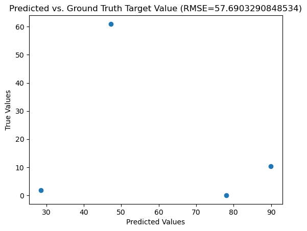
plot_rmse
This function will calculate the RMSE values and plot the expected vs predicted values for each value in the testing set, based on the model created with the training data.
results= plot_rmse("data/energy_train.csv", "data/energy_test.csv", "results/lin_reg_results.png")